Problem
Needed to convert a numeric representation of weekday to words. In Google Sheets the WEEKDAY function returns a number from 1-7 representing Sunday-Saturday. Google's documentation recommends using the TEXT function to format a date into words, but what if I wanted a different format other than the shortform (i.e. Mon) or the longform (i.e. Monday), such as "MO" for Monday.
Solution
A simple VLOOKUP would allow me to list out the numbers 1-7 and then the corresponding day of the week in the exact text that I want. But it seems a bit silly just to have a few cells kicking around dedicated to this. It turns out the range option does not need to reference specific cells, you can supply it an array table (data between curly braces)
Where column B is a timestamp, I customized the day of the week format like this:
=ARRAYFORMULA(VLOOKUP(WEEKDAY(B2:B),{1, "SU"; 2, "MO"; 3, "TU"; 4, "WE"; 5, "TH"; 6, "FR"; 7, "SA"},2))
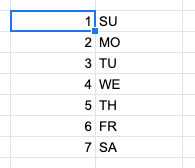
In the curly braces, the comma , indicates column break, and the semi-colon ; indicates row break. If you input just the curly braces part of the formula into a cell, you would get this:
={1, "SU"; 2, "MO"; 3, "TU"; 4, "WE"; 5, "TH"; 6, "FR"; 7, "SA"}
The Gist
Using VLOOKUP with an array table is a bit more complicated, but provides more flexibility -- say you needed the days in a different language, or you have some other data where you need to map one value to another