I often get data sets or survey responses where there is a column for categories, and in each cell the categories are separated by a comma. You might find something like this for movies data:
comedy, action, kids, animated
romance, action
documentaries, sports
If you had many rows with many categories then it wouldn't be so clear what all the categories are; and it's always more accurate to use a systematic approach than to eye-ball it.
Here's my approach
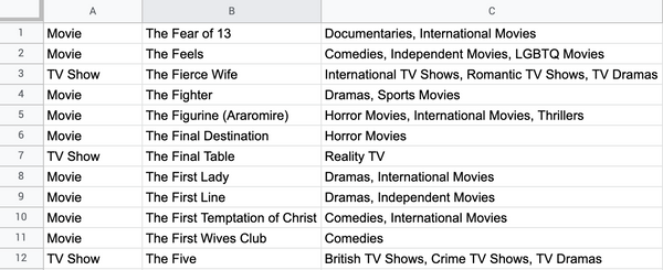
With the sample data, I want to get all the categories in column C

Final formula
For those who don't want the walk-thru here's the final formula I used in cell D1
=SORT(UNIQUE(FLATTEN(ARRAYFORMULA(SPLIT(C1:C12, ", ", FALSE)))))
The formula walk-thru
1. Separate out the categories by comma
In cell D1 input the formula
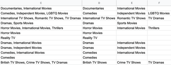
=ARRAYFORMULA(SPLIT(C1:C12, ", ", FALSE))
Using the SPLIT function we can split out the categories by comma. I'm using the optional FALSE flag for split_by_each so that I'm splitting by the comma and the space, otherwise the second category and beyond will start with a space. I could have instead leverage the TRIM function instead. I'm splitting all 12 rows with just one formula by using ARRAYFORMULA, I didn't want to fill down, you'll see why later. Notice that the categories fill up the columns D, E, F

2. Flatten out columns D, E, F into one column
Update the cell in D1 to this one
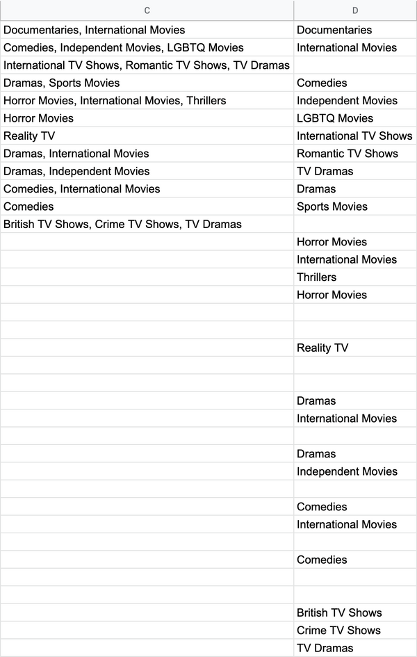
=FLATTEN(ARRAYFORMULA(SPLIT(C1:C12, ", ", FALSE)))
I can't always be certain how many columns the categories will get split out into. In the sample data the max number of categories per movie/show appears to be 3, but there could be more or less if I had a different data set. That's why I use the FLATTEN formula so all the categories are in one column. This is also why I used ARRAYFORMULA: the FLATTEN formula can take all the split out categories as the range (I didn't have to explicitly say the range is columns D, E, F). Now all the categories are in column D, but there are duplicates

3. Get unique categories and sort them alphabetically
Update the cell in D1 to this one
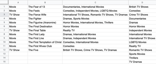
=SORT(UNIQUE(FLATTEN(ARRAYFORMULA(SPLIT(C1:C12, ", ", FALSE)))))
The UNIQUE formula takes the results from the FLATTEN formula (everything you see in column D in the image above) and only shows the unique categories. Then I sorted that list alphabetically by wrapping the SORT formula around everything. Now column D shows all the unique categories for the sample data
